A step-by-step example with the PFOA male-rat PBK model (Jaqpot model 1730)

Physiologically based kinetic (PBK) models have become an essential tool for understanding the absorption, distribution, metabolism and excretion (ADME) of chemicals and materials in living organisms. They provide a mechanistic link between external exposure and internal concentrations in target tissues, offering valuable insights for toxicology, pharmacology and regulatory decision-making.

At Jaqpot, we are committed to making advanced computational models accessible, transparent and easy to integrate into real-world research and regulatory workflows. That is why PBK models can be hosted directly on the Jaqpot platform, enabling scientists and regulators to run complex simulations without local installation, coding expertise or specialised software.

Jaqpot provides a cloud-native environment where PBK models are available to users. Researchers can upload, share and run their models through standardised APIs, so results are reproducible and methods transparent.

How It Works

Preparing the model in R

Developers write their PBK model in R using the well-known deSolve package, which is widely used for solving systems of ordinary differential equations (ODEs) and is a natural backbone for kinetic modelling. The model is then deployed to Jaqpot, where our team ensures it runs securely and reproducibly, so users can execute it in the cloud without worrying about dependencies or local installations.

To make a model "Jaqpot-ready", the R code must follow a specific structure. Let's walk through its building blocks using a model that is already live on Jaqpot: the extended PBK model for perfluorooctanoic acid (PFOA) in male rats (Tsiros et al., 2024), available at app.jaqpot.org/dashboard/models/1730. The model describes PFOA biodistribution after intravenous or oral administration across lungs, gonads, brain, heart, stomach, intestines, liver, spleen, kidney and a lumped "rest of body" compartment, connected through arterial and venous plasma (Figure 1). The complete R code of this example is available on GitHub: github.com/ntua-unit-of-control-and-informatics/PBK_Grouping.

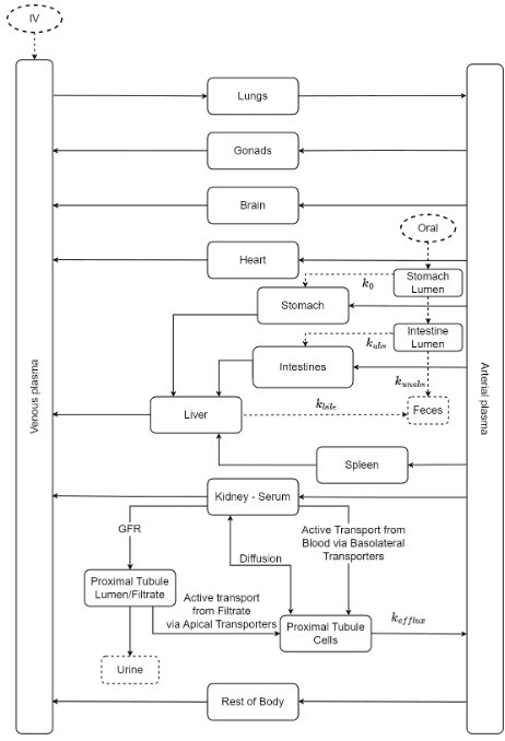
Figure 1. Structure of the extended PFOA male-rat PBK model, with the oral and intravenous administration routes and the kidney sub-model.

Step 1 — user_input

This defines what goes into the model. For the PFOA model, the user provides four inputs:

• the body weight of the rat (BW, kg);
• the administration route (admin.type: "iv" or "oral");
• the administration time(s) (admin.time, h);
• the administered dose(s) (admin.dose, mg).

BW <- 0.2            # kg
admin.type <- "oral" # "iv" or "oral"
admin.dose <- 1      # mg
user_input <- list("BW" = BW, "admin.type" = admin.type,
                   "admin.time" = 0.0001, "admin.dose" = admin.dose)

Step 2 — create.params(user_input)

This function turns the inputs into the full set of parameters the ODEs need, both constant and input-dependent.

Example: The PFOA model combines rat physiological data (cardiac output, blood-flow fractions and tissue volumes from Brown et al., 1997 and Davies & Morris, 1993) with PFOA-specific parameters: tissue:blood partition coefficients (Kudo et al., 2007), the free fraction of PFOA in plasma, kinetic constants of the renal transporters (basolateral OAT1/OAT3 and apical Oatp1a1, extrapolated from in vitro data), and rate constants for gastric emptying, intestinal absorption, and biliary and urinary elimination. Flows and rate constants are then scaled allometrically to the body weight provided by the user.

create.params <- function(user_input){
  with(as.list(user_input), {
    # Physiological parameters (Brown 1997; Davies 1993)
    QCC = 14.0        # cardiac output (L/h/kg^0.75)
    QkidneyC = 0.141  # fraction of cardiac output to kidney
    VliverC = 0.0366  # liver volume (L/kg BW)
    ...

    # Chemical-specific parameters
    MW = 414.07       # PFOA molecular mass (g/mol)
    Pliver = 2.2      # liver:blood partition coefficient (Kudo 2007)
    Free = 0.09       # free fraction in plasma
    ...

    # Scaling to the user's body weight
    QC <- QCC*(BW^0.75)*(1-Htc)  # cardiac output, plasma (L/h)
    Vliver = VliverC*BW          # liver volume (L)
    kbile = kbilec*BW^(-0.25)    # biliary elimination (1/h)
    ...

    return(list("QC" = QC, "Vliver" = Vliver, "kbile" = kbile, ...,
                "admin.type" = admin.type,
                "admin.time" = admin.time, "admin.dose" = admin.dose))
  })
}

Step 3 — create.inits()

Here you set the starting values of the state variables.

Example: The PFOA model tracks 24 state variables – the amount of PFOA in each tissue, in arterial and venous plasma, in the kidney sub-compartments (kidney blood, proximal tubule cells, filtrate), in the stomach and intestinal lumen, and in urine and faeces. All start at zero, because PFOA enters the body only through the dosing events defined in the next step.

create.inits <- function(parameters){
  with(as.list(parameters), {
    Arest <- 0; Aliver <- 0; APTC <- 0; Afil <- 0;
    Astomach_lumen <- 0; Aven_free <- 0; Aart_free <- 0; ...
    return(c("Arest" = Arest, "Aliver" = Aliver, ...,
             "Aven_free" = Aven_free, "Aart_free" = Aart_free))
  })
}

Step 4 — create.events()

Events introduce time-dependent changes, such as single or repeated dosing.

Example: Each dose is added at its administration time either to the venous plasma (intravenous) or to the stomach lumen (oral). Supplying several times and doses creates a dosing schedule; the function checks that their numbers match.

create.events <- function(parameters){
  with(as.list(parameters), {
    if (length(admin.time) != length(admin.dose)){
      stop("The times of administration should be equal in number to the doses")
    }
    if (admin.type == "iv"){
      events <- list(data = data.frame(var = "Aven_free", time = admin.time,
                                       value = admin.dose, method = "add"))
    } else if (admin.type == "oral"){
      events <- list(data = data.frame(var = "Astomach_lumen", time = admin.time,
                                       value = admin.dose, method = "add"))
    } else {
      stop("The type of administration should be either iv or oral")
    }
    return(events)
  })
}

Step 5 — custom.func()

An optional function for any extra calculations the ODEs need. The PFOA model does not use it, so it simply returns nothing.

custom.func <- function(){
  return()
}

Step 6 — ode.func()

This is the heart of the model. It contains the mass-balance equations that govern the kinetics over time, written in a format compatible with deSolve.

Example: The PFOA model contains 24 equations. Most tissues are flow-limited: their uptake depends on blood flow, the partition coefficient and the free fraction in plasma. The kidney is described in more detail, with glomerular filtration, saturable (Michaelis–Menten) basolateral and apical transport into the proximal tubule cells, efflux back to the blood and urinary elimination. Oral doses pass from the stomach lumen to the intestine and are absorbed to the liver, which also eliminates PFOA through bile. Besides the derivatives, the function returns the organ concentrations that users will see, and a mass-balance check (Atotal) that should equal the total dose.

ode.func <- function(time, inits, params, custom.func){
  with(as.list(c(inits, params)), {
    Cart = (Aart_free/Vart_plasma)/Free  # total PFOA in arterial plasma (mg/L)
    Cfil = Afil/Vfil                     # concentration in filtrate (mg/L)
    ...
    # Flow-limited tissue, e.g. heart
    dAheart = Qheart*(Cart - CVheart)*Free
    # Saturable apical reabsorption from filtrate into tubule cells
    dA_apical <- (Vmax_apical*Cfil)/(Km_apical + Cfil)
    # Filtrate: glomerular filtration - reabsorption - urine
    dAfil = Cart*GFR*Free - dA_apical - Afil*kurine
    ...
    list(c("dAheart" = dAheart, "dAfil" = dAfil, ...),
         "Cplasma_ven" = Aven_free/Vven_plasma/Free,
         "Cliver" = Aliver/Vliver, ...)
  })
}

Deploying the model

Finally, the model developer decides which outputs will be visible in Jaqpot's user interface. For the PFOA model these are the PFOA concentrations in venous and arterial plasma, liver, kidneys, brain, intestine, testis, spleen, heart, lung, stomach and carcass.

Once everything is set, the model is uploaded to Jaqpot with the deploy.pbpk() function of the jaqpotr R package. Our team then reviews and completes the deployment to make sure everything is secure and ready to use.

predicted.feats <- c("Cplasma_ven", "Cplasma_art", "Cliver", "Ckidneys",
                     "Cbrain", "Cintestine", "Ctestis", "Cspleen",
                     "Cheart", "Clung", "Cstomach", "Ccarcass")

# Deploy the model on the Jaqpot server to create a web service
deploy.pbpk(user.input = user_input, out.vars = predicted.feats,
            create.params = create.params, create.inits = create.inits,
            create.events = create.events, custom.func = custom.func,
            ode.fun = ode.func, envFile = ".env")

That's it! With these steps, your PBK model moves from R code to a fully deployed, interactive simulation on Jaqpot.

Running the model

Once hosted, the model can be run through the graphical user interface or accessed programmatically through Jaqpot's open API. In the Predict tab of the PFOA model, the user sets the body weight, the administration route, the dose(s) and the simulation window – no line of code needed. Figure 2 shows a simulation for a 0.5 kg male rat receiving a single oral dose of 0.1 mg PFOA.

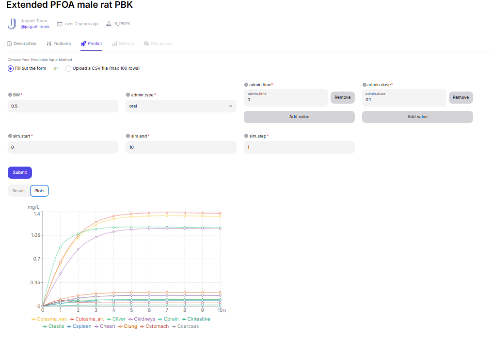
Figure 2. Running the PFOA model in the Jaqpot interface: the input form and the predicted organ concentration–time profiles.

Outputs and visualisation

The same simulation can be run from Python with the Jaqpot SDK (Figure 3), giving identical results (Figure 4) – so a workflow tested in the browser can move into an automated pipeline without re-implementation.

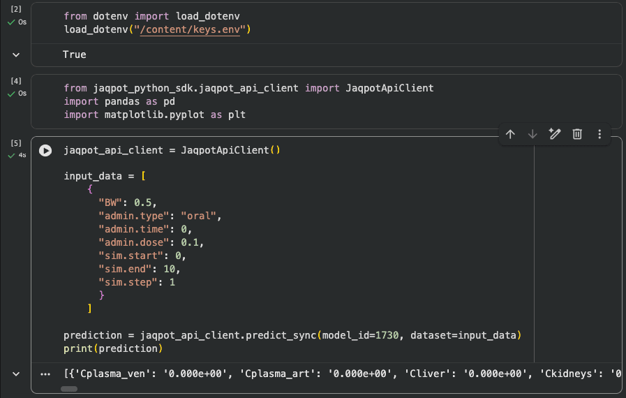
Figure 3. Running the PFOA model programmatically with the Jaqpot Python SDK.

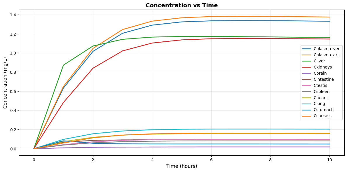
Figure 4. Concentration–time profiles returned by the programmatic run, identical to those from the graphical interface.

Applications

• Drug development: predict pharmacokinetics in animals and humans.
• Chemical safety assessment: simulate internal concentrations from external exposures – for example, the organ burden of persistent PFAS such as PFOA.
• SSbD workflows: combine PBK simulations with hazard predictions to inform design choices early in the innovation cycle.

Getting Started

Try it yourself

1. Create a free account at jaqpot.org.
2. Browse the available models – such as the PFOA model – or deploy your own.
3. Run simulations directly from your browser or through API calls.
4. See the full R code of the PFOA example on GitHub.

Looking Ahead

Our vision is to make PBK modelling as seamless and collaborative as possible. By hosting these models in Jaqpot, we are lowering barriers to adoption and fostering a community where researchers, industry and regulators can work together to improve chemical and drug safety.

If you are developing PBK models, we invite you to host them on Jaqpot and contribute to an open, transparent and FAIR modelling ecosystem.

Reference

Tsiros P, Minadakis V, Li D, Sarimveis H. Parameter grouping and co-estimation in physiologically based kinetic models using genetic algorithms. Toxicological Sciences 2024;200(1):31–46. doi:10.1093/toxsci/kfae051